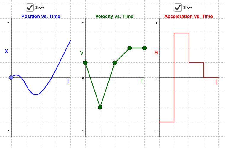
So, you’ve got this graph. A Position vs. Time graph. It looks like a squiggly line, and your teacher wants you to turn it into a Velocity vs. Time graph. Whoa, hold on—let’s not panic.
Think of it like this: you’re a detective, and this graph is telling you a story about motion. Your job? To translate that story into a new language. And guess what? It’s way easier than it sounds.
The First Graph: Where Are You?
Picture your friend walking across a giant football field. You’re timing them. A Position vs. Time graph shows where they are at each second. If the line is flat, they’re just standing there, probably checking their phone.
Must Read
If the line goes up steeply, they’re sprinting. If it goes up slowly, they’re taking a lazy stroll. Slope is everything here. The slope of this line tells you the speed—or, more precisely, the velocity.
Enter the Slope: Your New Best Friend
Here’s the secret: the slope of a Position vs. Time graph is the velocity. It’s math’s way of being logical. If the line is a straight, upward diagonal, the slope is constant—so the velocity is constant. Easy peasy.
But what if the line is curved? Oh, you’re in for a treat. A curve means the slope is changing. That means acceleration is happening. Like when you push a shopping cart and then let go—the speed changes, and the line curves.
The Transformation: From Position to Velocity
Now, take that slope information and plop it onto a new graph. This one has Velocity on the y-axis and Time on the x-axis. For every point on your position graph, ask yourself: “What’s the slope here?”
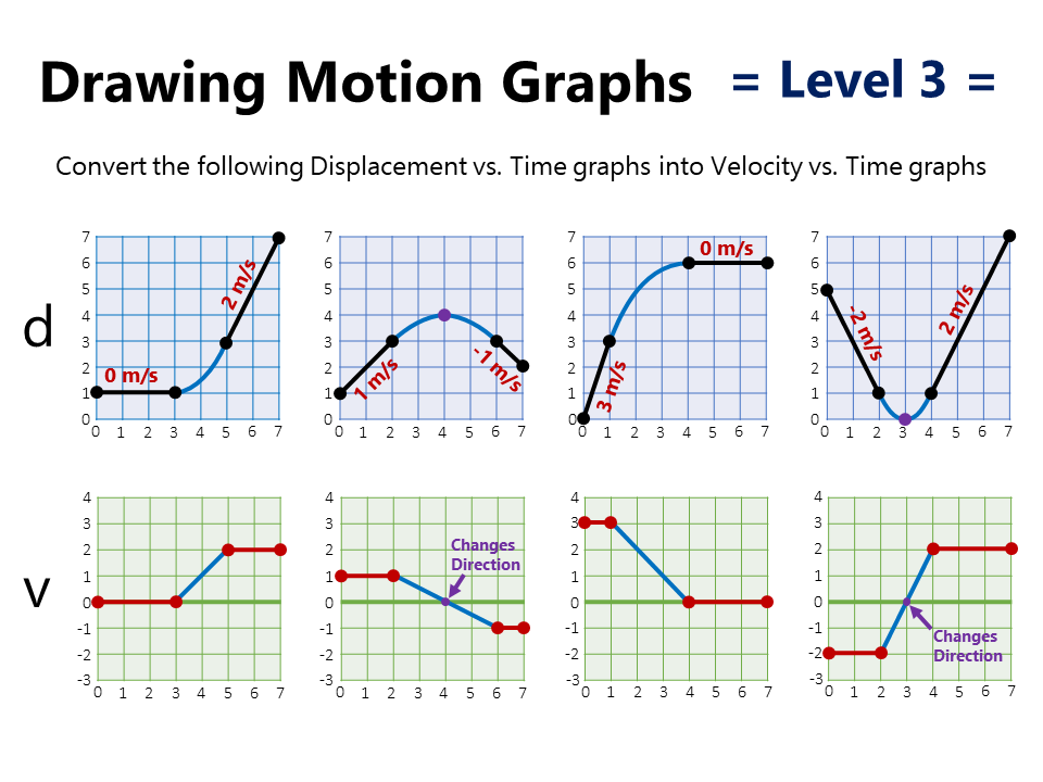
If the position graph is a straight, flat line (slope = 0), your velocity graph is a flat horizontal line at zero. “You’re not moving, buddy.”
If the position graph is a steep upward line (big positive slope), your velocity graph is a high flat line. If the position graph is a downhill slope (negative slope), your velocity graph dips below zero. Yes, negative velocity means you’re going backward. Don’t be embarrassed—happens to the best of us.
 Velocity Time Graph And Position Time Graphs
When the Graph Gets Fancy: Curves & Corners
Let’s say your position graph is a parabola—like a smiley face. That means the slope starts steep, then gets less steep, then goes flat at the top. So your velocity graph is a straight diagonal line that starts high and goes down to zero. Mind blown yet?
And if the position graph has a sharp corner (like a V-shape)? That means the slope changes instantly. Your velocity graph will have a jump—a sudden change. It’s like your friend stops dead and turns around. No smooth transitions; just a hard stop. Kind of like realizing you forgot your keys.
Real-Life Example: The Coffee Run
Imagine you walk to the coffee shop. Your position graph starts flat (you’re at home), then goes up (you walk), then goes flat again (you’re in line), then goes down (you walk back). What does the velocity graph look like?
First part: zero velocity (flat line at zero). Second part: positive constant velocity (flat line above zero). Third part: zero velocity again (flat line at zero). Fourth part: negative constant velocity (flat line below zero). Boom—you just turned a story into numbers.
Common Jokes (and Mistakes)
People often think that distance traveled is the same as velocity. Nope. Velocity cares about direction. If you go forward then backward, your velocity graph might average out to zero, but you still walked a ton. It’s like running on a treadmill—tons of work, zero net movement.
Also, don’t confuse the shape of the position graph with the shape of the velocity graph. A curved position graph doesn’t give you a curved velocity graph—it gives you a straight one if the curve is a parabola. Physics is sneaky like that.
 Velocity Time Graph And Position Time Graphs PhysicsLAB: Constant
Why Bother? Because You’re a Time Traveler… Sort Of
When you convert a position graph to a velocity graph, you’re basically watching the past and predicting the future. If you know how fast something is going right now, you can guess where it will be a second later. It’s like being a fortune teller, but with math.
Plus, this skill unlocks the next level: velocity to acceleration graphs. And those help you understand why your car lurches when you hit the gas. It’s all connected—like a weird, beautiful family tree of motion.
The Big Reveal: It’s Just Subtraction with Steps
Here’s the cheater’s way to do it: between two times, find the change in position (Δx) and the change in time (Δt). Then velocity = Δx / Δt. Do that for every pair of points. Plot each result. You are now a graph wizard.
Practice on a few simple graphs: a straight line, a curve, a flat line. In ten minutes, you’ll be able to look at any position graph and imagine its velocity twin. It’s like learning to see in a new color.
Wrapping Up: You’ve Got This
So next time your physics teacher drops a Position vs. Time graph on your desk, don’t sweat it. Just whisper to yourself, “I see the slope. I see the story. I will make the velocity graph my loyal companion.”
Remember, every graph is just a conversation between the past and the present. And you’re the translator. So go ahead, draw those lines, and smile—because you’re literally turning locations into motion.
And if you mess up? No big deal. Even the best physicists sometimes graph wrong—they just call it “data collecting.” Keep practicing, keep laughing, and know that every time you convert a graph, you’re one step closer to understanding the universe. Plus, you’ll look really cool doing it.😊